 |
| The bust of Paul Dirac at Princeton University's Fine Hall Library I snapped Apr. 23, 2012 |
"Although Dirac did not at first fully appreciate what his own equation was telling him, his resolute faith in the logic of mathematics as a means to physical reasoning, his explanation of spin as a consequence of the union of quantum mechanics and special relativity, and the eventual discovery of the positron, represents one of the great triumphs of theoretical physics."
From Wiki:
In physics, more specifically relativistic quantum mechanics, the Dirac equation[1] is a wave equation, formulated by Britishphysicist Paul Dirac in 1928. It provided a description of elementary spin-½ particles, such as electrons, consistent with both the principles of quantum mechanics and the theory of special relativity, and made relativistic corrections to quantum mechanics. It accounted for the fine structure of the hydrogen spectrum in a rigorous way. The equation also implied the existence of a new form of matter, antimatter, hitherto unsuspected and unobserved, later discovered experimentally. It also provided a theoreticaljustification for the introduction of several-component wave functions in Pauli's phenomenological theory of spin. Although Dirac did not at first fully appreciate what his own equation was telling him, his resolute faith in the logic of mathematics as a means to physical reasoning, his explanation of spin as a consequence of the union of quantum mechanics and special relativity, and the eventual discovery of the positron, represents one of the great triumphs of theoretical physics.
Contents[hide] |
[edit]The Dirac equation
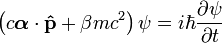
where ψ = ψ(r, t) is a complex four-component field ψ that Dirac thought of as the wave function for the electron, r and t are the space and time coordinates, m is the rest massof the electron,  is the momentum operator, c is the speed of light, and ħ is the reduced Planck constant (h/2π). Furthermore, α is a vector operator whose components are 4 × 4 matricies: α = (α1, α2, α3), and β is another 4 × 4 matrix.
is the momentum operator, c is the speed of light, and ħ is the reduced Planck constant (h/2π). Furthermore, α is a vector operator whose components are 4 × 4 matricies: α = (α1, α2, α3), and β is another 4 × 4 matrix.
This single symbolic equation unravels into four coupled linear first-order partial differential equations for the four quantities that make up the field. These matrices, and the form of the field, have a deep mathematical significance. The algebraic structure represented by the Dirac matrices had been created some 50 years earlier by the English mathematician W. K. Clifford. In turn, Clifford's ideas had emerged from the mid-19th century work of the German mathematician Hermann Grassmann in his "Lineale Ausdehnungslehre" (Theory of Linear Extensions). The latter had been regarded as well-nigh incomprehensible by most of his contemporaries. The appearance of something so seemingly abstract, at such a late date, and in such a direct physical manner, is one of the most remarkable chapters in the history of physics.
Dirac's purpose in casting this equation was to explain the behavior of the relativistically moving electron, and so to allow the atom to be treated in a manner consistent with relativity. His rather modest hope was that the corrections introduced this way might have bearing on the problem of atomic spectra. Up until that time, attempts to make the old quantum theory of the atom compatible with the theory of relativity by discretizing the angular momentum of the electron's orbit had failed - and the new quantum mechanics ofHeisenberg, Pauli, Jordan, Schrödinger, and Dirac himself had not developed sufficiently to treat this problem. Although Dirac's original intentions were satisfied, his equation had far deeper implications for the structure of matter, and introduced new mathematical classes of objects that are now essential elements of fundamental physics.
[edit]Background and development
[edit]Making the Schrödinger equation relativistic
The Dirac equation was motivated by the Schrödinger equation for a massive free particle:

The left side, the non-relativistic kinetic energy, is the square of the momentum operator divided by twice the mass m. Relativity treats space and time as a unified spacetime, so a relativistic generalization of this equation requires that space and time derivatives must enter symmetrically, as they do in the Maxwell equations that govern the behavior of light — the equations must be differentially of the same order in space and time. In relativity, the momentum and the energy are the space and time parts of a space-time vector, the 4-momentum, and they are related by the relativistically invariant relation

which says that the length of this vector is proportional to the invariant mass m. Substituting the operator equivalents of the energy and momentum from the Schrödinger theory, we get an equation describing the propagation of waves, constructed from relativistically invariant objects, the Klein-Gordon equation:

where the wave function ψ is a relativistic scalar: a complex number which has the same numerical value in all frames of reference. The space and time derivatives both enter to second order. This has an important consequence for the interpretation of the equation: the expression for the density is no longer positive definite - the initial values of both ψ and  may be freely chosen, and the density may thus become negative, something that is impossible if the density is to be a legitimate probability density, as it is for the Schrödinger equation. Thus we cannot get a relativistic generalization of the Schrödinger equation under the naive assumption that the wave function is a scalar.
may be freely chosen, and the density may thus become negative, something that is impossible if the density is to be a legitimate probability density, as it is for the Schrödinger equation. Thus we cannot get a relativistic generalization of the Schrödinger equation under the naive assumption that the wave function is a scalar.
Although the Klein-Gordon equation is not a successful relativistic generalization of the Schrödinger equation, this equation is a valid field equation in the context of quantum field theory, describing a spinless particle field (e.g. pi meson). Historically, Schrödinger himself arrived at this equation before the one that bears his name, but soon discarded it. In the context of quantum field theory, the indefinite density is understood to correspond to the charge density, which can be positive or negative, and not the probability density. Finding a relativistic field equation with first order derivatives required a more elaborate construction.
[edit]Square root of the Klein-Gordon equation
Dirac thought to try an equation that was first order in both space and time. One could, for example, formally take the relativistic expression for the energy
 ,
,
expand the square root in an infinite series, replace p and E by their operator equivalents, set up an eigenvalue problem, then solve the equation formally by iterations. Most physicists had little faith in such a formidable process, even if it were technically possible.
As the story goes, Dirac was staring into the fireplace at Cambridge, pondering this problem, when he hit upon the idea of taking the square root of the wave operator thus:

On multiplying out the right side, it can be noticed that the cross-terms, such as  , will vanish if we assume that for every different pair of coefficents theiranticommutator vanishes:
, will vanish if we assume that for every different pair of coefficents theiranticommutator vanishes:![[A,B]_+ = 0, [A,C]_+ = 0, \cdots \, ,](http://upload.wikimedia.org/wikipedia/en/math/8/9/f/89fe6cb86cf53b9f5c753803ac21bef4.png)
where the brackets [, ]+ denote the anticommutator:
![[A,B]_+ = AB + BA \,](http://upload.wikimedia.org/wikipedia/en/math/f/7/a/f7ad33578fe04c0ddc8ba54b6198d92d.png)
and that they each square to the 4 × 4 identity:

Dirac, who had just then been intensely involved with working out the foundations of Heisenberg's matrix mechanics, immediately understood that these conditions could be met if A, B, C and D are matrices, with the implication that the wave function has multiple components. This immediately explained the appearance of two-component wave functions in Pauli's phenomenological theory of spin, something that up until then had been regarded as mysterious, even to Pauli himself. However, one needs at least 4 × 4 matrices to set up a system with the properties required — so the wave function had four components, not two, as in the Pauli theory, or one, as in the bare Schrödinger theory. The four-component wave function represents a new class of mathematical object in physical theories, spinors, that makes its first appearance here.
Given the factorization in terms of these matrices, the Dirac equation can be obtained from one of the factors, an equation first order in space and time (as given above).
[show]Derivation
[edit]Mathematical formulation
The Dirac equation can take several different forms, relating to the nature of the matrices.
[edit]The Dirac α and β matrices
Starting from the original form of Dirac's equation:
The matrices α1, α2, α3, and β, are 4 × 4 matrices. Some properties are as follows:
They are all Hermitian so that the Dirac Hamiltonian is Hermitian.
They have squares equal to the 4 × 4 identity matrix I4:

and they all mutually anticommute:
![[\alpha_i,\alpha_j]_+ = 0 \,](http://upload.wikimedia.org/wikipedia/en/math/b/4/5/b456d01cdf2de95c5a5834f9356b5f6a.png)
![[\alpha_i,\beta]_+ = 0 \,](http://upload.wikimedia.org/wikipedia/en/math/e/d/8/ed8ee081141d1f39a868f1abf4dd93e3.png)
for all i and j not equal to each other.
Dirac defined these matrices (in the chiral representation) as the following:[4]

NB: In the literature and this context, all matrices are usually written in italic like scalars, bold is used for a vector whose components are matrices. Superscript and subscript indices are used to label components of the vectors of matrices. See Covariance and contravariance of vectors - except for identity matrices. Also it is conventional not to write identity matrices, or write them as 1, as they can be revealed from their positions in the equation. If a matrix is shown as 2 × 2 when it is known to be 4 × 4, then the missing identities are the 2 × 2 identity matrix, I2. If no matrix is shown at all in the full Dirac equation, then it is understood that the missing identity is 4 × 4 identity matrix, I4.
[edit]The Dirac γ matrices
It is useful to define new matrices:[3]


These matrices are known as the gamma matrices, and there are many different representations of them. In the Pauli-Dirac representation (and basis):
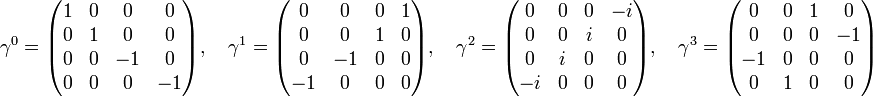
While in the chiral representation (and basis), also known as the Weyl representation:

and the spatial gamma matrices are the same as in the Pauli-Dirac representation. The gamma matrices are representative basis elements of a Clifford algebra, satisfying the defining relationship

in which  is the Minkowski metric of signature (+---). Using gamma matrices, the Dirac equation becomes:
is the Minkowski metric of signature (+---). Using gamma matrices, the Dirac equation becomes:
This is a particularly useful way to write the equation, since it can be immediately translated into the language of 4-vectors and relativistic covariance can be demonstrated (see below), while it resembles a similar form to the original.
[edit]The Pauli spin σ matrices
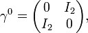
The Dirac matrices are block matrices; where the partitions are the 2 × 2 zero matrix, the 2 × 2 Identity matrix I2, and the Pauli matrices σx, σy, σz (equivalently written σ1, σ2,σ3). In practice these rather large matrices can be written in the following standard representations: the α and β matrices are

the Pauli-Dirac basis is

and the chiral basis is:
where  are as before.
are as before.
These can be written in terms of the Kronecker product (aka direct product, denoted by  or sometimes
  )[5][6] of the matrices
or sometimes )[5][6] of the matrices
and

where

is a vector whose components are the Pauli matrices.
The Dirac equation can then be written directly in terms of the Pauli σ matrices, illustrating how the Dirac theory accounts for Pauli's theory of spin. Substituting the α and βmatrices leads to

[show]Proof of equivalence
[edit]Dirac equation in curved spacetime
The Dirac equation in curved spacetime can be written by using vierbein fields and the gravitational spin connection. The vierbein defines a local rest frame, allowing the constant Dirac matrices to act at each spacetime point. In this way, Dirac's equation takes the following form in curved spacetime[7]:

 is the
  is the
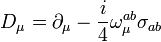
where  is the commutator of Dirac matrices:
is the commutator of Dirac matrices:![\sigma_{ab}=\frac{i}{2} \left[\gamma_{a},\gamma_{b}\right]](http://upload.wikimedia.org/wikipedia/en/math/9/1/4/91483818aedf428ca45d4af9251ae3bd.png)
and  are the spin connection components.
are the spin connection components.
Note that here Latin indices denote the "Lorentzian" vierbein labels while Greek indices denote manifold coordinate indices.
[edit]Physical interpretation
The Dirac theory, while providing a wealth of information that is accurately confirmed by experiments, nevertheless introduces a new physical paradigm that appears at first difficult to interpret and even paradoxical. Some of these issues of interpretation must be regarded as open questions. The Dirac theory brilliantly answered some of the outstanding issues in physics at the time it was put forward, while posing others that are still the subject of debate. Many of these issues were resolved in modern quantum field theory by considering the Dirac equation not as a relativistic description of quantum mechanics but merely as another relativistic field equation, on the same footing as the Klein-Gordon equation or Maxwell's equations, in which ψ is not interpreted as a wave function but rather as a fermion field, similar to the Klein-Gordon scalar field or electromagnetic field. Nevertheless, considering Dirac's equation as a relativistic version of Schrödinger's equation is extremely computationally useful, and raises important issues.
[edit]Identification of observables
The critical physical question in a quantum theory is - what are the physically observable quantities defined by the theory? According to general principles, such quantities are defined by Hermitian operators that act on the Hilbert space of possible states of a system. The eigenvalues of these operators are then the possible results of measuring the corresponding physical quantity. In the Schrödinger theory, the simplest such object is the overall Hamiltonian, which represents the total energy of the system. If we wish to maintain this interpretation on passing to the Dirac theory, we must take the Hamiltonian to be
![H = \gamma^0 \left [ mc^2 + c \sum_{k = 1}^3 \gamma^k \left ( p_k-\frac{q}{c}A_k \right ) \right ] + qA^0.](http://upload.wikimedia.org/wikipedia/en/math/e/0/2/e0246468a405e774241b975194f88085.png)
This looks promising, because we see by inspection the rest energy of the particle and, in case A = 0, the energy of a charge placed in an electric potential qA0. What about the term involving the vector potential? In classical electrodynamics, the energy of a charge moving in an applied potential is

Thus the Dirac Hamiltonian is fundamentally distinguished from its classical counterpart, and we must take great care to correctly identify what is an observable in this theory. Much of the apparent paradoxical behavior implied by the Dirac equation amounts to a misidentification of these observables. The following issues arise with the Dirac equation, which are not immediately easy to interpret:
Klein paradox: when a Dirac electron interacts with an electric potential, the total probability is not conserved. Also, the electron can tunnel into high potential barriers, unlike the case in quantum mechanics as described by the Schrödinger equation.
Zitterbewegung: there is an apparent fluctuation (at the speed of light) of the position of an electron around the median.
[edit]Hole theory
The negative E solutions of Dirac's equation were problematic, for it was assumed that the particle has a positive energy. Mathematically, however, there seemed to be no reason to reject the negative-energy solutions. Since they exist, we cannot simply ignore them, for once we include the interaction between the electron and the electromagnetic field, any electron placed in a positive-energy eigenstate would decay into negative-energy eigenstates of successively lower energy by emitting excess energy in the form of photons. Real electrons obviously do not behave in this way.
To cope with this problem, Dirac introduced the hypothesis, known as hole theory: that the vacuum is the many-body quantum state in which all the negative-energy electron eigenstates are occupied. This description of the vacuum as a "sea" of electrons is called the Dirac sea. Since the Pauli exclusion principle forbids electrons from occupying the same state, any additional electron would be forced to occupy a positive-energy eigenstate, and positive-energy electrons would be forbidden from decaying into negative-energy eigenstates.
Dirac further reasoned that if the negative-energy eigenstates are incompletely filled, each unoccupied eigenstate – called a hole – would behave like a positively charged particle. The hole possesses a positive energy, since energy is required to create a particle–hole pair from the vacuum. As noted above, Dirac initially thought that the hole might be the proton, but Hermann Weyl pointed out that the hole should behave as if it had the same mass as an electron, whereas the proton is over 1800 times heavier. The hole was eventually identified as the positron, experimentally discovered by Carl Anderson in 1932.
It is not entirely satisfactory to describe the "vacuum" using an infinite sea of negative-energy electrons. The infinitely negative contributions from the sea of negative-energy electrons has to be canceled by an infinite positive "bare" energy and the contribution to the charge density and current coming from the sea of negative-energy electrons is exactly canceled by an infinite positive "jellium" background so that the net electric charge density of the vacuum is zero. In quantum field theory, a Bogoliubov transformationon the creation and annihilation operators (turning an occupied negative-energy electron state into an unoccupied positive energy positron state and an unoccupied negative-energy electron state into an occupied positive energy positron state) allows us to bypass the Dirac sea formalism even though, formally, it is equivalent to it.
In certain applications of condensed matter physics, however, the underlying concepts of "hole theory" are valid. The sea of conduction electrons in an electrical conductor, called a Fermi sea, contains electrons with energies up to the chemical potential of the system. An unfilled state in the Fermi sea behaves like a positively-charged electron, though it is referred to as a "hole" rather than a "positron". The negative charge of the Fermi sea is balanced by the positively-charged ionic lattice of the material.
[edit]Properties
[edit]Covariant form and relativistic invariance
Main articles: Covariance and contravariance of vectors and relativistic invariance
To demonstrate the relativistic invariance of the equation, it is advantageous to cast it into a form in which the space and time derivatives appear on an equal footing. Using the gamma-matrix form above, the covariant form can be obtained by inserting the gradient operator and collecting all space and time derivatives together (dividing by c for convenience):

then using the 4-position (as above) and (+−−−) metric signature to gain the contraction between the gamma matrices and the 4-position derivatives;

so we have[8]

Using the Feynman slash notation the equation becomes

This covariant form has further relativistic implications:
- the Dirac equation is the square root of the Klein-Gordon equation. The Klein-Gordon equation is based on
 , meaning the Dirac equation is based on its square root
  .
. - Any solution to the Dirac equation is automatically a solution to the Klein-Gordon equation, but not vice versa, i.e. there are solutions to the Klein-Gordon equation that do not solve the Dirac equation.[3]
This can be found by factoring the Klein-Gordon equation (in the slash notation):
![0 = [\hbar^2\partial^\mu \partial_\mu + (mc)^2]\psi = [(\hbar\partial\!\!\!/)^2 + (mc)^2]\psi = (i\hbar\partial\!\!\!/ + mc)(-i\hbar\partial\!\!\!/ + mc)\psi \,.](http://upload.wikimedia.org/wikipedia/en/math/2/5/f/25f43c1a22b15c86cf12fcafafd60bf3.png)
and noticing the last factor,  , is simply the Dirac equation. In this sense, the Dirac equation takes an extra step forward into relativistic quantum mechanics compared with Klein–Gordon equation.
, is simply the Dirac equation. In this sense, the Dirac equation takes an extra step forward into relativistic quantum mechanics compared with Klein–Gordon equation.
The complete system is summarized using the Minkowski metric on spacetime in the form
![[\gamma^\mu,\gamma^\nu ]_+ = 2 g^{\mu\nu} \,](http://upload.wikimedia.org/wikipedia/en/math/4/b/2/4b28fd3b8889337069a4fddc546b1f39.png)
where again [, ]+ denotes the anticommutator. These are the defining relations of a Clifford algebra over a pseudo-orthogonal 4-d space with metric signature (+−−−). The specific Clifford algebra employed in the Dirac equation is known today as the Dirac algebra. Although not recognized as such by Dirac at the time the equation was formulated, in hindsight the introduction of this geometric algebra also represents a step forward in the development of relativistic quantum theory.
[edit]Relativistic eigenvalue equation
See also: eigenvalue
Further, the 4-momentum vector is

so inserting the quantum operators obtains the 4-momentum operator;

(the −iħ becomes +iħ preceding the 3-momentum operator). Contraction of this operator with the gamma matrices (using Feynman slash notation) gives

which dramatically shortens the Dirac equation to the familiar structure of momentum;

The Dirac equation may now be interpreted as an eigenvalue equation, where the rest mass is proportional to an eigenvalue of the 4-momentum operator, the proportionality constant being the speed of light c.
[edit]Spinor transformations
Main article: spinors
In practice, physicists often use units of measure such that ħ = c = 1, known as "natural units". The equation then takes the simple form
A fundamental theorem states that if two distinct sets of matrices are given that both satisfy the Clifford relations, then they are connected to each other by a similarity transformation:

If in addition the matrices are all unitary, as are the Dirac set, then S itself is unitary;

The transformation U is unique up to a multiplicative factor of absolute value 1. Let us now imagine a Lorentz transformation to have been performed on the space and time coordinates, and on the derivative operators, which form a covariant vector. For the operator  to remain invariant, the gammas must transform among themselves as a contravariant vector with respect to their spacetime index. These new gammas will themselves satisfy the Clifford relations, because of the orthogonality of the Lorentz transformation. By the fundamental theorem, we may replace the new set by the old set subject to a unitary transformation. In the new frame, remembering that the rest mass is a relativistic scalar, the Dirac equation will then take the form
to remain invariant, the gammas must transform among themselves as a contravariant vector with respect to their spacetime index. These new gammas will themselves satisfy the Clifford relations, because of the orthogonality of the Lorentz transformation. By the fundamental theorem, we may replace the new set by the old set subject to a unitary transformation. In the new frame, remembering that the rest mass is a relativistic scalar, the Dirac equation will then take the form

If we now define the transformed spinor

then we have the transformed Dirac equation in a way that demonstrates manifest relativistic invariance:

Thus, once we settle on any unitary representation of the gammas, it is final provided we transform the spinor according to the unitary transformation that corresponds to the given Lorentz transformation. The various representations of the Dirac matrices employed will bring into focus particular aspects of the physical content in the Dirac field (see below). The representation shown here is known as the standard representation - in it, the upper two components go over into Pauli's 2-spinor wave function in the limit of low energies and small velocities in comparison to light.
The considerations above reveal the origin of the gammas in geometry, harking back to Grassmann's original motivation - they represent a fixed basis of unit vectors in spacetime. Similarly, products of the gammas such as  represent oriented surface elements, and so on. With this in mind, we can find the form of the unit volume element in spacetime in terms of the gammas as follows. By definition, it is
represent oriented surface elements, and so on. With this in mind, we can find the form of the unit volume element in spacetime in terms of the gammas as follows. By definition, it is
For this to be an invariant, the epsilon symbol must be a tensor, and so must contain a factor of  , where g is the determinant of the metric tensor. Since this is negative, that factor is imaginary. Thus
, where g is the determinant of the metric tensor. Since this is negative, that factor is imaginary. Thus
This matrix is given the special symbol  , owing to its importance when one is considering improper transformations of spacetime, that is, those that change the orientation of the basis vectors. In the standard representation it is
, owing to its importance when one is considering improper transformations of spacetime, that is, those that change the orientation of the basis vectors. In the standard representation it is
This matrix will also be found to anticommute with the other four Dirac matrices. It takes on a leading role when questions of parity arise, because the volume element as a directed magnitude changes sign under a space-time reflection. Taking the positive square root above thus amounts to choosing a handedness convention on space-time.
[edit]Adjoint equation and probability conservation
Main articles: Conservation of probability and probability current
In the Schrödinger theory, the probability density is given by the positive definite expression

and this density is convected according to the probability current vector

according to a continuity equation for probability. For a relativistic theory, these may be incorporated into a probability 4-current, which has the relativistically covariant expression

where (translating usual cartesian-subscript notation into vector indices):[3]

By defining the adjoint spinor

 is the
  , and noticing that
 ,
,
we obtain, by taking the Hermitian conjugate of the Dirac equation and multiplying from the right by  , the adjoint equation:
, the adjoint equation:
where  is understood to act to the left. Multiplying the Dirac equation by
  from the left, and the adjoint equation by
  from the right, and subtracting, produces the law of conservation of the Dirac current:
is understood to act to the left. Multiplying the Dirac equation by from the left, and the adjoint equation by from the right, and subtracting, produces the law of conservation of the Dirac current: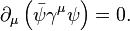
Now we see the great advantage of the first-order equation over the one Schrödinger had tried - this is the conserved current density required by relativistic invariance, only now its 4th component is positive definite and thus suitable for the role of a probability density:

Because the probability density now appears as the fourth component of a relativistic vector, and not a simple scalar as in the Schrödinger equation, it will be subject to the usual effects of the Lorentz transformations such as time dilation. Thus for example atomic processes that are observed as rates, will necessarily be adjusted in a way consistent with relativity, while those involving the measurement of energy and momentum, which themselves form a relativistic vector, will undergo parallel adjustment which preserves the relativistic covariance of the observed values.
In a general case (if a certain linear function of electromagnetic field does not vanish identically), three out of four components of the spinor function in the Dirac equation can be algebraically eliminated, yielding an equivalent fourth-order partial differential equation for just one component. Furthermore, this remaining component can be made real by a gauge transform.[9]
[edit]See also
- Bohr–Sommerfeld theory
- Breit equation
- Dirac field
- Einstein-Maxwell-Dirac equations
- Feynman checkerboard
- Foldy–Wouthuysen transformation
- Klein–Gordon equation
- Quantum electrodynamics
- Rarita–Schwinger equation
- Theoretical and experimental justification for the Schrödinger equation
- Dirac equation in the algebra of physical space
- EPR paradox
- The Dirac Equation appears on the floor of Westminster Abbey. It appears on the plaque commemorating Paul Dirac's life which was inaugurated on November 13, 1995.[10]
[edit]References
- ^ B Hatfield, Quantum Field Theory of Point Particles and Strings, Addison-Wesley, Reading, MA, 1989.
- ^ Particle Physics (3rd Edition), B. R. Martin, G.Shaw, Manchester Physics Series, John Wiley & Sons, ISBN 978-0-470-03294-7
- ^ a b c d Quantum Field Theory, D. McMahon, Mc Graw Hill (USA), 2008, ISBN 978-0-07-154382-8
- ^ Quantum Mechanics, E. Abers, Pearson Ed., Addison Wesley, Prentice Hall Inc, 2004, ISBN 978-0-13-146100-0
- ^ http://mathworld.wolfram.com/KroneckerProduct.html
- ^ Encyclopaedia of Physics (2nd Edition), R.G. Lerner, G.L. Trigg, VHC publishers, 1991, (Verlagsgesellschaft) 3-527-26954-1, (VHC Inc.) 0-89573-752-3
- ^ Lawrie, Ian D.. A Unified Grand Tour of Theoretical Physics.
- ^ The Cambridge Handbook of Physics Formulas, G. Woan, Cambridge University Press, 2010, ISBN 978-0-521-57507-2
- ^ Journal of Mathematical Physics, 52, 082303 (2011) (http://jmp.aip.org/resource/1/jmapaq/v52/i8/p082303_s1 or http://akhmeteli.org/wp-content/uploads/2011/08/JMAPAQ528082303_1.pdf )
- ^ http://www.dirac.ch/PaulDirac.html
[edit]Selected papers
- Dirac, P. A. M. (1928). "The Quantum Theory of the Electron". Proceedings of the Royal Society A: Mathematical, Physical and Engineering Sciences 117 (778): 610.doi:10.1098/rspa.1928.0023.
- P.A.M. Dirac "The Quantum Theory of the Electron", Proc. R. Soc. A117) link to the volume of the Proceedings of the Royal Society of London containing the article at page 610
- P.A.M. Dirac "A Theory of Electrons and Protons", Proc. R. Soc. A126) link to the volume of the Proceedings of the Royal Society of London containing the article at page 360
- C.D. Anderson, Phys. Rev. 43, 491 (1933)
- R. Frisch and O. Stern, Z. Phys. 85, 4 (1933)
[edit]Textbooks
- Halzen, Francis; Martin, Alan (1984). Quarks & Leptons: An Introductory Course in Modern Particle Physics. John Wiley & Sons. ISBN.
- Dirac, P.A.M., Principles of Quantum Mechanics, 4th edition (Clarendon, 1982)
- Shankar, R., Principles of Quantum Mechanics, 2nd edition (Plenum, 1994)
- Bjorken, J D & Drell, S, Relativistic Quantum mechanics
- Thaller, B., The Dirac Equation, Texts and Monographs in Physics (Springer, 1992)
- Schiff, L.I., Quantum Mechanics, 3rd edition (McGraw-Hill, 1968)
- Griffiths, D.J., Introduction to Elementary Particles, 2nd edition (Wiley-VCH, 2008) ISBN 978-3-527-40601-2.
[edit]External links
- The Dirac Equation at MathPages
- The Nature of the Dirac Equation, its solutions and Spin
- Dirac equation for a spin ½ particle
- Pedagogic Aids to Quantum Field Theory click on Chap. 4 for a step-by-small-step introduction to the Dirac equation, spinors, and relativistic spin/helicity operators.
- Nature of spinors Introductory explanation of spinors.