- Note: General relativity articles using tensors will use the abstract index notation.
Why tensors?
The principle of general covariance states that the laws of physics should take the same mathematical form in all reference frames and was one of the central principles in the development of general relativity. The term 'general covariance' was used in the early formulation of general relativity, but is now referred to by many as diffeomorphism covariance. Although diffeomorphism covariance is not the defining feature of general relativity[1], and controversies remain regarding its present status in GR, the invariance property of physical laws implied in the principle coupled with the fact that the theory is essentially geometrical in character (making use of non-Euclidian geometry) suggested that general relativity be formulated using the language of tensors. This will be discussed further below.Spacetime as a manifold
Main articles: Spacetime and Spacetime topology
Most modern approaches to mathematical general relativity begin with the concept of a manifold. More precisely, the basic physical construct representing gravitation - a curved spacetime - is modelled by a four-dimensional, smooth, connected, Lorentzian manifold. Other physical descriptors are represented by various tensors, discussed below.The rationale for choosing a manifold as the fundamental mathematical structure is to reflect desirable physical properties. For example, in the theory of manifolds, each point is contained in a (by no means unique) coordinate chart and can be thought of as representing the 'local spacetime' around the observer (represented by the point). The principle of local Lorentz covariance, which states that the laws of special relativity hold locally about each point of spacetime, lends further support to the choice of a manifold structure for representing spacetime, as locally around a point on a general manifold, the region 'looks like', or approximates very closely Minkowski space (flat spacetime).
The idea of coordinate charts as 'local observers who can perform measurements in their vicinity' also makes good physical sense, as this is how one actually collects physical data - locally. For cosmological problems, a coordinate chart may be quite large.
Local versus global structure
An important distinction in physics is the difference between local and global structures. Measurements in physics are performed in a relatively small region of spacetime and this is one reason for studying the local structure of spacetime in general relativity, whereas determining the global spacetime structure is important, especially in cosmological problems.An important problem in general relativity is to tell when two spacetimes are 'the same', at least locally. This problem has its roots in manifold theory where determining if two Riemannian manifolds of the same dimension are locally isometric ('locally the same'). This latter problem has been solved and its adaptation for general relativity is called the Cartan-Karlhede algorithm.
Tensors in GR
Further information: Tensor, Tensor (intrinsic definition), Classical treatment of tensors, and Intermediate treatment of tensors
One of the profound consequences of relativity theory was the abolition of privileged reference frames. The description of physical phenomena should not depend upon who does the measuring - one reference frame should be as good as any other. Special relativity demonstrated that no inertial reference frame was preferential to any other inertial reference frame, but preferred inertial reference frames over noninertial reference frames. General relativity eliminated preference for inertial reference frames by showing that there is no preferred reference frame (inertial or not) for describing nature.Any observer can make measurements and the precise numerical quantities obtained only depend on the coordinate system used. This suggested a way of formulating relativity using 'invariant structures', those that are independent of the coordinate system (represented by the observer) used, yet still have an independent existence. The most suitable mathematical structure seemed to be a tensor. For example, when measuring the electric and magnetic fields produced by an accelerating charge, the values of the fields will depend on the coordinate system used, but the fields are regarded as having an independent existence, this independence represented by the electromagnetic field tensor .
Mathematically, tensors are generalised linear operators - multilinear maps. As such, the ideas of linear algebra are employed to study tensors.
At each point
 of a manifold, the tangent and cotangent spaces to the manifold at that point may be constructed. Vectors (sometimes referred to as contravariant vectors) are defined as elements of the tangent space and covectors (sometimes termed covariant vectors, but more commonly dual vectors or one-forms) are elements of the cotangent space.
At
, these two vector spaces may be used to construct type  tensors, which are real-valued multilinear maps acting on the direct sum of
  copies of the cotangent space with
  copies of the tangent space. The set of all such multilinear maps forms a vector space, called the tensor product space of type at and denoted by
  . If the tangent space is n-dimensional, it can be shown that
 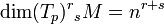 .
.In the general relativity literature, it is conventional to use the component syntax for tensors.
A type (r,s) tensor may be written as

where
 is a basis for the i-th tangent space and
  a basis for the j-th cotangent space.
As spacetime is assumed to be four-dimensional, each index on a tensor can be one of four values. Hence, the total number of elements a tensor possesses equals 4R, where R is the sum of the numbers of covariant and contravariant indices on the tensor (a number called the rank of the tensor).
Symmetric and antisymmetric tensors
Main articles: Antisymmetric tensor and Symmetric tensor
Some physical quantities are represented by tensors not all of whose components are independent. Important examples of such tensors include symmetric and antisymmetric tensors. Antisymmetric tensors are commonly used to represent rotations (for example, the vorticity tensor).Although a generic rank R tensor in 4 dimensions has 4R components, constraints on the tensor such as symmetry or antisymmetry serve to reduce the number of distinct components. For example, a symmetric rank two tensor T satisfies Tab = Tba and possesses 10 independent components, whereas an antisymmetric (skew-symmetric) rank two tensor P satisfies Pab = -Pba and has 6 independent components. For ranks greater than two, the symmetric or antisymmetric index pairs must be explicitly identified.
Antisymmetric tensors of rank 2 play important roles in relativity theory. The set of all such tensors - often called bivectors - forms a vector space of dimension 6, sometimes called bivector space.
The metric tensor
Main article: Metric tensor (general relativity)
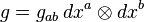
The metric tensor is a central object in general relativity that describes the local geometry of spacetime (as a result of solving the Einstein field equation). Using the weak-field approximation, the metric can also be thought of as representing the 'gravitational potential'. The metric tensor is often just called 'the metric'.The metric is a symmetric tensor and is an important mathematical tool. As well as being used to raise and lower tensor indices, it also generates the connections which are used to construct the geodesic equations of motion and the Riemann curvature tensor.
A convenient means of expressing the metric tensor in combination with the incremental intervals of coordinate distance that it relates to is through the line element:

This way of expressing the metric was used by the pioneers of differential geometry. While some relativists consider the notation to be somewhat old-fashioned, many readily switch between this and the alternative notation:
The metric tensor is commonly written as a 4 by 4 matrix. Due to the symmetry of the metric, this matrix is symmetric and has 10 independent components.
Invariants
One of the central features of GR is the idea of invariance of physical laws. This invariance can be described in many ways, for example, in terms of local Lorentz covariance, the general principle of relativity, or diffeomorphism covariance.A more explicit description can be given using tensors. The crucial feature of tensors used in this approach is the fact that (once a metric is given) the operation of contracting a tensor of rank R over all R indices gives a number - an invariant - that is independent of the coordinate chart one uses to perform the contraction. Physically, this means that if the invariant is calculated by any two observers, they will get the same number, thus suggesting that the invariant has some independent significance. Some important invariants in relativity include:
- The Ricci scalar:

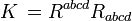
- The Kretschmann scalar:
Tensor classifications
The classification of tensors is a purely mathematical problem. In GR, however, certain tensors that have a physical interpretation can be classified with the different forms of the tensor usually corresponding to some physics. Examples of tensor classifications useful in general relativity include the Segre classification of the energy-momentum tensor and the Petrov classification of the Weyl tensor. There are various methods of classifying these tensors, some of which use tensor invariants.Tensor fields in GR
Main article: Tensor field
Tensor fields on a manifold are maps which attach a tensor to each point of the manifold. This notion can be made more precise by introducing the idea of a fibre bundle, which in the present context means to collect together all the tensors at all points of the manifold, thus 'bundling' them all into one grand object called the tensor bundle. A tensor field is then defined as a map from the manifold to the tensor bundle, each point p being associated with a tensor at p.The notion of a tensor field is of major importance in GR. For example, the geometry around a star is described by a metric tensor at each point, so at each point of the spacetime the value of the metric should be given to solve for the paths of material particles. Another example is the values of the electric and magnetic fields (given by the electromagnetic field tensor) and the metric at each point around a charged black hole to determine the motion of a charged particle in such a field.
Vector fields are contravariant rank one tensor fields. Important vector fields in relativity include the four-velocity,
 , which is the coordinate distance travelled per unit of proper time, the four-acceleration
  and the four-current
  describing the charge and current densities. Other physically important tensor fields in relativity include the following:
- The stress-energy tensor
 , a symmetric rank-two tensor.
 - The electromagnetic field tensor
 , a rank-two antisymmetric tensor.
At each point of a spacetime on which a metric is defined, the metric can be reduced to the Minkowski form using Sylvester's Law of Inertia.
Tensorial derivatives
Before the advent of general relativity, changes in physical processes were generally described by partial derivatives, for example, in describing changes in electromagnetic fields (see Maxwell's equations). Even in special relativity, the partial derivative is still sufficient to describe such changes. However, in general relativity, it is found that derivatives which are also tensors must be used. The derivatives have some common features including that they are derivatives along integral curves of vector fields.The problem in defining derivatives on manifolds that are not flat is that there is no natural way to compare vectors at different points. An extra structure on a general manifold is required to define derivatives. Below are described two important derivatives that can be defined by imposing an additional structure on the manifold in each case.
Affine connections
Main article: Affine connection
The curvature of a spacetime can be characterised by taking a vector at some point and parallel transporting it along a curve on the spacetime. An affine connection is a rule which describes how to legitimately move a vector along a curve on the manifold without changing its direction.By definition, an affine connection is a bilinear map
 , where
  is a space of all vector fields on the spacetime. This bilinear map can be described in terms of a set of connection coefficients (also known as Christoffel symbols) specifying what happens to components of basis vectors under infinitesimal parallel transport:
Despite their tempting appearance, the connection coefficients are not the components of a tensor.
Generally speaking, there are D3 independent connection coefficients at each point of spacetime. The connection is called symmetric if
 . A symmetric connection has D2(D+1)/2 coefficients.
For any curve γ and two points A = γ(0) and B = γ(t) on this curve, an affine connection gives rise to a map of vectors in the tangent space at A into vectors in the tangent space at B:
 ,
,and
 can be computed component-wise by solving the differential equation
 being the vector tangent to the curve at the point γ(t).
An important affine connection in general relativity is the Levi-Civita connection, which is a symmetric connection obtained from parallel transporting a tangent vector along a curve whilst keeping the inner product of that vector constant along the curve. The resulting connection coefficients (Christoffel symbols) can be calculated directly from the metric. For this reason, this type of connection is often called a metric connection.
The covariant derivative
Main article: Covariant derivative
Let X be a point,  a vector located at X, and
  a vector field. The idea of differentiating at X along the direction of in a physically meaningful way can be made sense of by choosing an affine connection and a parameterized smooth curve
  such that
  and
and  . The formula
for a covariant derivative of
along associated with connection  turns out to give curve-independent results and can be used as a "physical definition" of a covariant derivative.
It can be expressed using connection coefficients:

The expression in brackets, called a covariant derivative of X (with respect to the connection) and denoted by
 , is more often used in calculations:
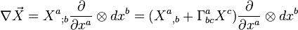
A covariant derivative of X can thus be viewed as a differential operator acting on a vector field sending it to a type (1,1) tensor ('increasing the covariant index by 1') and can be generalised to act on type (r,s) tensor fields sending them to type (r, s+1) tensor fields. Notions of parallel transport can then be defined similarly as for the case of vector fields. By definition, a covariant derivative of a scalar field is equal to the regular derivative of the field.
In the literature, there are three common methods of denoting covariant differentiation:

Many standard properties of regular partial derivatives also apply to covariant derivatives:


 , if c is a constant
In General Relativity, one usually refers to "the" covariant derivative, which is the one associated with Levi-Civita affine connection. By definition, Levi-Civita connection preserves the metric under parallel transport, therefore, the covariant derivative gives zero when acting on a metric tensor (as well as its inverse). It means that we can take the (inverse) metric tensor in and out of the derivative and use it to raise and lower indices:

The Lie derivative
Main articles: Lie derivative and Spacetime symmetries
Another important tensorial derivative is the Lie derivative. Whereas the covariant derivative required an affine connection to allow comparison between vectors at different points, the Lie derivative uses a congruence from a vector field to achieve the same purpose. The idea of Lie dragging a function along a congruence leads to a definition of the Lie derivative, where the dragged function is compared with the value of the original function at a given point. The Lie derivative can be defined for type (r,s) tensor fields and in this respect can be viewed as a map that sends a type (r,s) to a type (r,s) tensor.The Lie derivative is usually denoted by
 , where X is the vector field along whose congruence the Lie derivative is taken.
The Lie derivative of any tensor along a vector field can be expressed through the covariant derivatives of that tensor and vector field. (In fact, any derivative will work, but covariant derivative is convenient because it commutes with raising and lowering indices.) The Lie derivative of a scalar is just the directional derivative:


 which is equivalent to
The Riemann curvature tensor
Main article: Riemann tensor (general relativity)
A crucial feature of general relativity is the concept of a curved manifold. A useful way of measuring the curvature of a manifold is with an object called the Riemann (curvature) tensor.This tensor measures curvature by use of an affine connection by considering the effect of parallel transporting a vector between two points along two curves. The discrepancy between the results of these two parallel transport routes is essentially quantified by the Riemann tensor.
This property of the Riemann tensor can be used to describe how initially parallel geodesics diverge. This is expressed by the equation of geodesic deviation and means that the tidal forces experienced in a gravitational field are a result of the curvature of spacetime.
Using the above procedure, the Riemann tensor is defined as a type (1,3) tensor and when fully written out explicitly contains the Christoffel symbols and its first partial derivatives. The Riemann tensor has 20 independent components. The vanishing of all these components over a region indicates that the spacetime is flat in that region. From the viewpoint of geodesic deviation, this means that initially parallel geodesics in that region of spacetime will stay parallel.
The Riemann tensor has a number of properties sometimes referred to as the symmetries of the Riemann tensor. Of particular relevance to general relativity are the algebraic and differential Bianchi identities.
The connection and curvature of any Riemannian manifold are closely related, the theory of holonomy groups, which are formed by taking linear maps defined by parallel transport around curves on the manifold, providing a description of this relationship.
The energy-momentum tensor
Main article: Energy-momentum tensor (general relativity)
The sources of any gravitational field (matter and energy) are represented in relativity by a type (0,2) symmetric tensor called the energy-momentum tensor. It is closely related to the Ricci tensor. Being a second rank tensor in four dimensions, the energy-momentum tensor may be viewed as a 4 by 4 matrix. The various admissible matrix types, called Jordan forms cannot all occur, as the energy conditions that the energy-momentum tensor is forced to satisfy rule out certain forms.Energy conservation
In GR, there is a local law for the conservation of energy-momentum. It can be succinctly expressed by the tensor equation:
The corresponding statement of local energy conservation in special relativity is:

This illustrates the rule of thumb that 'partial derivatives go to covariant derivatives'.
The Einstein field equations
Main article: Einstein field equations
The Einstein field equations (EFE) are the core of general relativity theory. The EFE describe how mass and energy (as represented in the stress-energy tensor) are related to the curvature of space-time (as represented in the Einstein tensor). In abstract index notation, the EFE reads as follows:
The solutions of the EFE are metric tensors. The EFE, being non-linear differential equations for the metric, are often difficult to solve. There are a number of strategies used to solve them. For example, one strategy is to start with an ansatz (or an educated guess) of the final metric, and refine it until it is specific enough to support a coordinate system but still general enough to yield a set of simultaneous differential equations with unknowns that can be solved for. Metric tensors resulting from cases where the resultant differential equations can be solved exactly for a physically reasonable distribution of energy-momentum are called exact solutions. Examples of important exact solutions include the Schwarzschild solution and the Friedman-Lemaître-Robertson-Walker solution.
The EIH approximation plus other references (e.g. Geroch and Jang, 1975 - 'Motion of a body in general relativity', JMP, Vol. 16 Issue 1).
The geodesic equations
Main article: Geodesic (general relativity)
Once the EFE are solved to obtain a metric, it remains to determine the motion of inertial objects in the spacetime. In general relativity, it is assumed that inertial motion occurs along timelike and null geodesics of spacetime as parameterized by proper time. Geodesics are curves that parallel transport their own tangent vector  , i.e.
  . This condition - the geodesic equation - can be written in terms of a coordinate system xa with the tangent vector
  :
:
where
 , τ parametrises proper time along the curve and the presence of the Christoffel symbols is made manifest.
A principal feature of general relativity is to determine the paths of particles and radiation in gravitational fields. This is accomplished by solving the geodesic equations.
The EFE relate the total matter (energy) distribution to the curvature of spacetime. Their nonlinearity leads to a problem in determining the precise motion of matter in the resultant spacetime. For example, in a system composed of one planet orbiting a star, the motion of the planet is determined by solving the field equations with the energy-momentum tensor the sum of that for the planet and the star. The gravitational field of the planet affects the total spacetime geometry and hence the motion of objects. It is therefore reasonable to suppose that the field equations can be used to derive the geodesic equations.
When the energy-momentum tensor for a system is that of dust, it may be shown by using the local conservation law for the energy-momentum tensor that the geodesic equations are satisfied exactly.
Lagrangian formulation
Main article: Variational methods in general relativity
The issue of deriving the equations of motion or the field equations in any physical theory is considered by many researchers to be appealing. A fairly universal way of performing these derivations is by using the techniques of variational calculus, the main objects used in this being Lagrangians.Many consider this approach to be an elegant way of constructing a theory, others as merely a formal way of expressing a theory (usually, the Lagrangian construction is performed after the theory has been developed).
Mathematical techniques for analyzing spacetimes
Having outlined the basic mathematical structures used in formulating the theory, some important mathematical techniques that are employed in investigating spacetimes will now be discussed.Frame fields
Main article: Frame fields in general relativity
A frame field is an orthonormal set of 4 vector fields (1 timelike, 3 spacelike) defined on a spacetime. Each frame field can be thought of as representing an observer in the spacetime moving along the integral curves of the timelike vector field. Every tensor quantity can be expressed in terms of a frame field, in particular, the metric tensor takes on a particularly convenient form. When allied with coframe fields, frame fields provide a powerful tool for analysing spacetimes and physically interpreting the mathematical results.Symmetry vector fields
Main article: Spacetime symmetries
Some modern techniques in analysing spacetimes rely heavily on using spacetime symmetries, which are infinitesimally generated by vector fields (usually defined locally) on a spacetime that preserve some feature of the spacetime. The most common type of such symmetry vector fields include Killing vector fields (which preserve the metric structure) and their generalisations called generalised Killing vector fields. Symmetry vector fields find extensive application in the study of exact solutions in general relativity and the set of all such vector fields usually forms a finite-dimensional Lie algebra.The Cauchy problem
Main article: Cauchy problem in general relativity
The Cauchy problem (sometimes called the initial value problem) is the attempt at finding a solution to a differential equation given initial conditions. In the context of general relativity, it means the problem of finding solutions to Einstein's field equations - a system of hyperbolic partial differential equations - given some initial data on a hypersurface. Studying the Cauchy problem allows one to formulate the concept of causality in general relativity, as well as 'parametrising' solutions of the field equations. Ideally, one desires global solutions, but usually local solutions are the best that can be hoped for. Typically, solving this initial value problem requires selection of particular coordinate conditions.Spinor formalism
Spinors find several important applications in relativity. Their use as a method of analysing spacetimes using tetrads, in particular, in the Newman-Penrose formalism is important.Another appealing feature of spinors in general relativity is the condensed way in which some tensor equations may be written using the spinor formalism. For example, in classifying the Weyl tensor, determining the various Petrov types becomes much easier when compared with the tensorial counterpart.
Regge calculus
Main article: Regge calculus
Regge calculus is a formalism which chops up a Lorentzian manifold into discrete 'chunks' (four-dimensional simplicial blocks) and the block edge lengths are taken as the basic variables. A discrete version of the Einstein-Hilbert action is obtained by considering so called 'deficit angles' of these blocks, a zero deficit angle corresponding to no curvature. This novel idea finds application in approximation methods in numerical relativity and quantum gravity, the latter using a generalisation of Regge calculus.Singularity theorems
Main article: Penrose-Hawking singularity theorems
| This section requires expansion. |
Numerical relativity
Main article: Numerical relativity
Numerical relativity is the sub-field of general relativity which seeks to solve Einstein's equations through the use of numerical methods. Finite difference, finite element and pseudo-spectral methods are used to approximate the solution to the partial differential equations which arise. Novel techniques developed by numerical relativity include the excision method and the puncture method for dealing with the singularities arising in black hole spacetimes. Common research topics include black holes and neutron stars.Perturbation methods
Main article: Perturbation methods in general relativity
| This section requires expansion. |
Notes
[1] The defining feature (central physical idea) of general relativity is that matter and energy cause the surrounding spacetime geometry to be curved.
References
- [1] Einstein, A. (1961). Relativity: The Special and General Theory. New York: Crown. ISBN 0-517-02961-8.
- [2] Misner, Charles; Thorne, Kip S. & Wheeler, John Archibald (1973). Gravitation. San Francisco: W. H. Freeman. ISBN 0-7167-0344-0.
- [3] Landau, L. D. and Lifshitz, E. M. (1975). Classical Theory of Fields (Fourth Revised English Edition). Oxford: Pergamon. ISBN 0-08-018176-7.
No comments:
Post a Comment